Design Of Experimenation
- Jan 9, 2023
- 5 min read
Updated: Feb 1, 2023
In this blog, I will cover what DOE is, my teams experience carrying out DOE using Full and Fractional factorial method, the case study with Full and Fractional method, and my reflection.
What is DOE?
A statistics-based approach to designing experiments.
A methodology to obtain knowledge of a complex, multi- variable process with the fewest trials possible.
An optimisation of the experimental process itself.
The backbone of any product design as well as any process/ product improvement efforts.
The main goal of using DOE is to determine which factors are most influential on an output. In this case for the practical, the output would be the flying distance of the ball.
There are 2 methods that come with DOE, Full and Fractional factorial methods. Fractional, as its name suggests, is where we only take a fraction of the number of runs. It is more efficient but less accurate.
PRACTICAL
Before commencing the practical, there was a pre-practical where we familiarised ourselves with DOE. We also had to identify the different variables of this practical.
Factors to test (dependent variables)
Arm Length
Projectile weight
Stop angle
Factor measured (independant variable)
Flying distance of projectile
8 replicates are done for each run
FULL FACTORIAL METHOD:
After obtaining all the data for 8 runs and 8 replicates, we had a total of 64 data points.

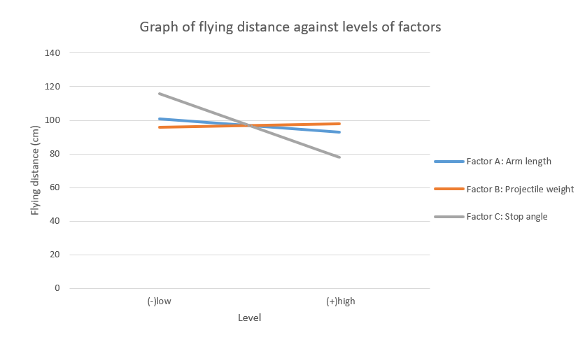
We used the calculated significance of main effects (solving for means) to plot the graph.
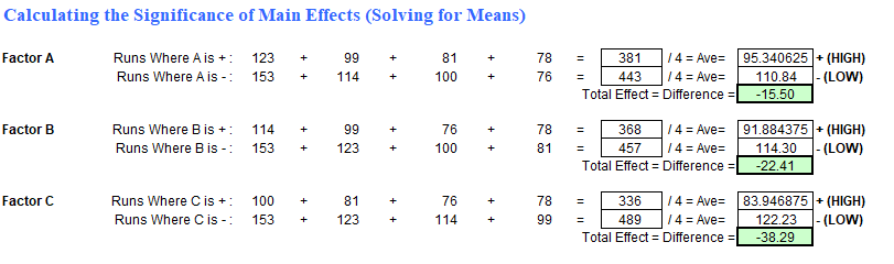
For example, to plot the line for Factor A, 2 points are needed. The first point's y value is taken from the average flying distance of when A is low, and the x value is low A.
The second point's y value is taken from the average flying distance of when A is high, and the x value is high A.
The same is done for plotting factor B and C with their respective average and low, hgih values.
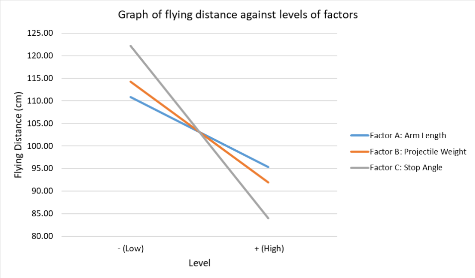
Based on gradient,

INTERACTION:
For the interactions, two factors are said to interact with each other if the effect of one factor on the response variable is different at different levels of the other factor.
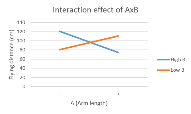
For this blog, I will go through the interaction between factor A and B
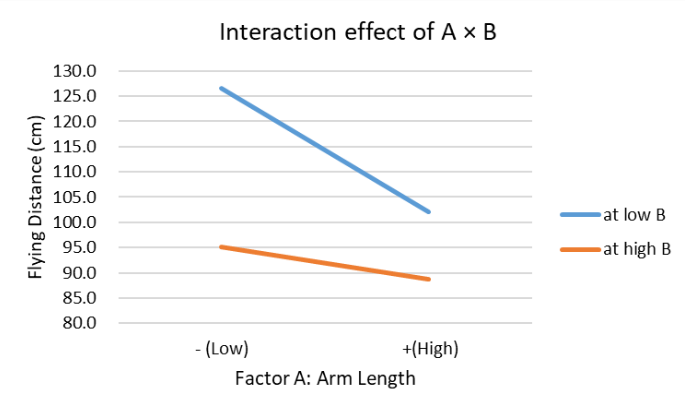
The first point of the blue line represents the average flying distance when B is low and A is low, the second point represents the average flying distance when B is low and A is high. Similarly with the orange line, but with high B.
The greater the difference between the gradients of the two plotted lines, the greater the interaction effect between factor A and B.
FRACTIONAL FACTORIAL METHOD:
Similar to full method, but with instead of 8 runs, we use 4 runs with 8 replicates. This gives us a total of 32 data points, half the original.
To choose the 4 runs, the combinations of high and low from each factor must appear the same number of times. In this case, each factor must have 2 lows and 2 highs in total for the 4 runs, with all the different combinations between each factor.

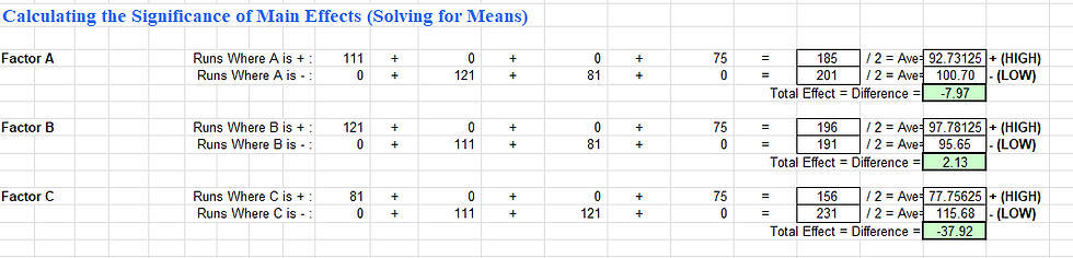
The method is similar to full factorial in terms of calculation, but faster and more susceptible to innaccuracy, as seen from the rating for each factor for fractional being different than for full factorial:

INTERACTION:
For fractional, it is the same method.
A larger difference in each gradient, the larger the interaction between the 2 factors.
Once we gathered all our data and analysed, we had a challenge to hit targets. It was quite challenging as we only had 2 tries to hit a target, and we had to use the data gathered to see which combination of factors would get the perfect distance to hit the target. It was very enjoyable though.
CASE STUDY
This case is studying the effect of 3 factors on the number of "bullets" (un-popped kernels) that remain at the bottom of the bag
Factors to test (dependent variables)
Diameter of bowls to contain the corn, 10 cm and 15 cm
Microwaving time, 4 minutes and 6 minutes
Power setting of microwave, 75% and 100%
Factor measured (independant variable)
Bullets, grams
8 runs were done.
FULL FACTORIAL:
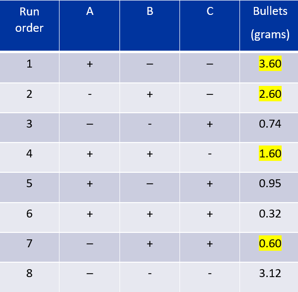
Using the excel provided previously, I keyed in the above values.

Taking the values seen in the image above for high and low of respective factors, we can plot the graph.
When diameter increases from 10cm to 15cm, the amount of bullets decreases from 1.77g to 1.62g
When microwaving time increases from 4min to 6min, the amount of bullets decreases from 2.10g to 1.28g.
When power increases from 75% to 100% , the amount of bullets decreases from 2.73g to 0.6525g.
Ranking is based on the gradient. Factor C has the largest gradient, Factor A has the smallest
Most significant- Factor C: Power
Factor B: Microwaving time
Least significant- Factor A: Diameter
This shows that when factor C varies, it has the most effect on the weight of bullets left after microwaving.
INTERACTIONS:
Interaction between factor A and factor B
At Low B,
Average of low A = 1.93g
Average of high A = 2.275g
Total effect of interaction = (2.275-1.93)g = 0.345g (increase)
At high B,
Average of low A = 1.6g
Average of high A = 0.96g
Total effect of interaction = (0.96-1.6)g = -0.64g (decrease)
The gradient of both lines are different, one is positive and the other is negative. Therefore there’s a significant interaction between A and B.
Interaction between factor A and factor C
At Low C,
Average of low A = 2.86g
Average of high A = 2.6g
Total effect of interaction = (2.6-2.86)g = -0.26g (decrease)
At high C,
Average of low A = 0.67g
Average of high A = 0.635g
Total effect of interaction = (0.635-0.67) = -0.035g (decrease)
The gradient of both lines are different by a very little margin.
Therefore there’s an interaction between A and C, but the interaction is extremely small.
Interaction between factor B and factor C.
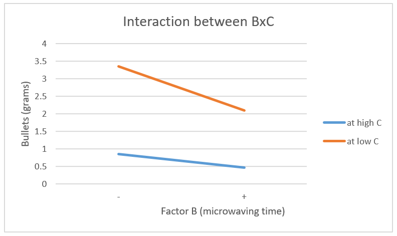
At Low C,
Average of low B = 3.36g
Average of high B = 2.1g
Average of high B = 2.g1tion = (2.1-3.36)g = -1.26g (decrease)
At High C,
Average of low B = 0.845g
Average of high B = 0.46g
Total effect of interaction = (0.46-0.845)g = - 0.385g(decrease)
The gradient of both lines are different by a little margin.
Therefore there’s an interaction between B and C, but the interaction is small.
FRACTIONAL FACTORIAL:
Runs 1,2,3,6 were chosen as they are orthogonal.

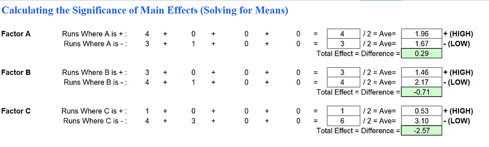
The graph was then plotted

When diameter increases from 10cm to 15cm, the amount of bullets increases from 1.67g to 1.96g
When microwaving time increases from 4min to 6min, the amount of bullets decreases from 2.17g to 1.46g.
When power increases from 75% to 100% , the amount of bullets decreases from 3.10g to 0.53g.
Ranking is based on the gradient. Factor C has the largest gradient, Factor A has the smallest
Most significant- Factor C: Power
Factor B: Microwaving time
Least significant- Factor A: Diameter
This shows that when factor C varies, it has the most effect on the weight of bullets left after microwaving.
The biggest difference between fractional and full is the effect factor A had on the bullets when diameter increased. For full, when factor A increased, number of bullets decreased, but for fractional, number of bullets increased.
excel sheet: DOE CPDD BLOG.xlsx
REFLECTION
DOE was a really interesting topic and a new way for me to experiment. I would say DOE is quite an accurate way to get reliable data for certain types of experiments that would have a certain number of factors affecting the measured factor. It's accurate in the sense that all the factors are fairly compared with one another, and we can also test for how the factors work together to affect the measured factor.
For the practical, it was definitely confusing at first and a little difficult to grasp the concept and calculations. But after going through the slides, it was easy to understand the concept. When it came to the interactions, it was also confusing to analyze what each graph meant with the different axes. But in the end, I understood after clarifying with some friends.
During the practical itself, it was quite fun and simple but very tedious as we had to get 64 measurements for full factorial and 32 measurements for fractional factorial, plus the fact that we had to do it in a different run order so that it was more fair. From the practical side, I definitely saw how the methods worked very well and gave us results immediately after all the data was collected. So I learned of a pretty reliable method for experimentation.
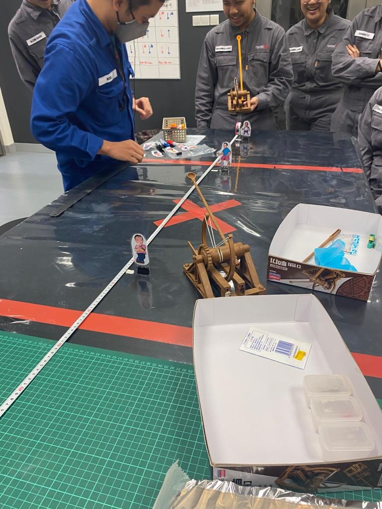
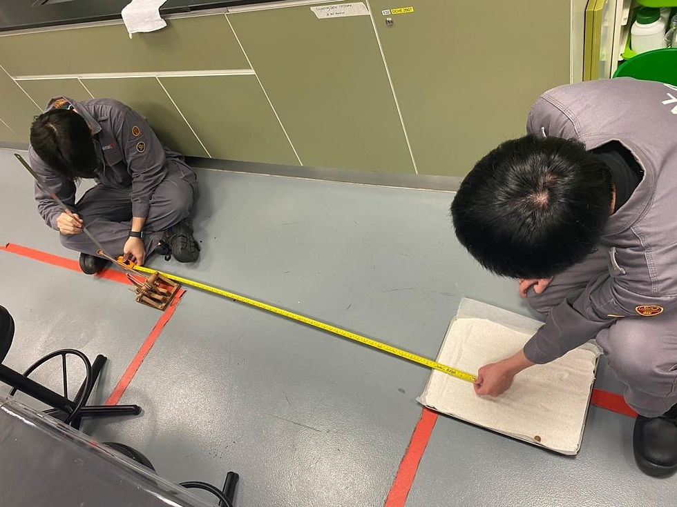
How measurement was done


Comments